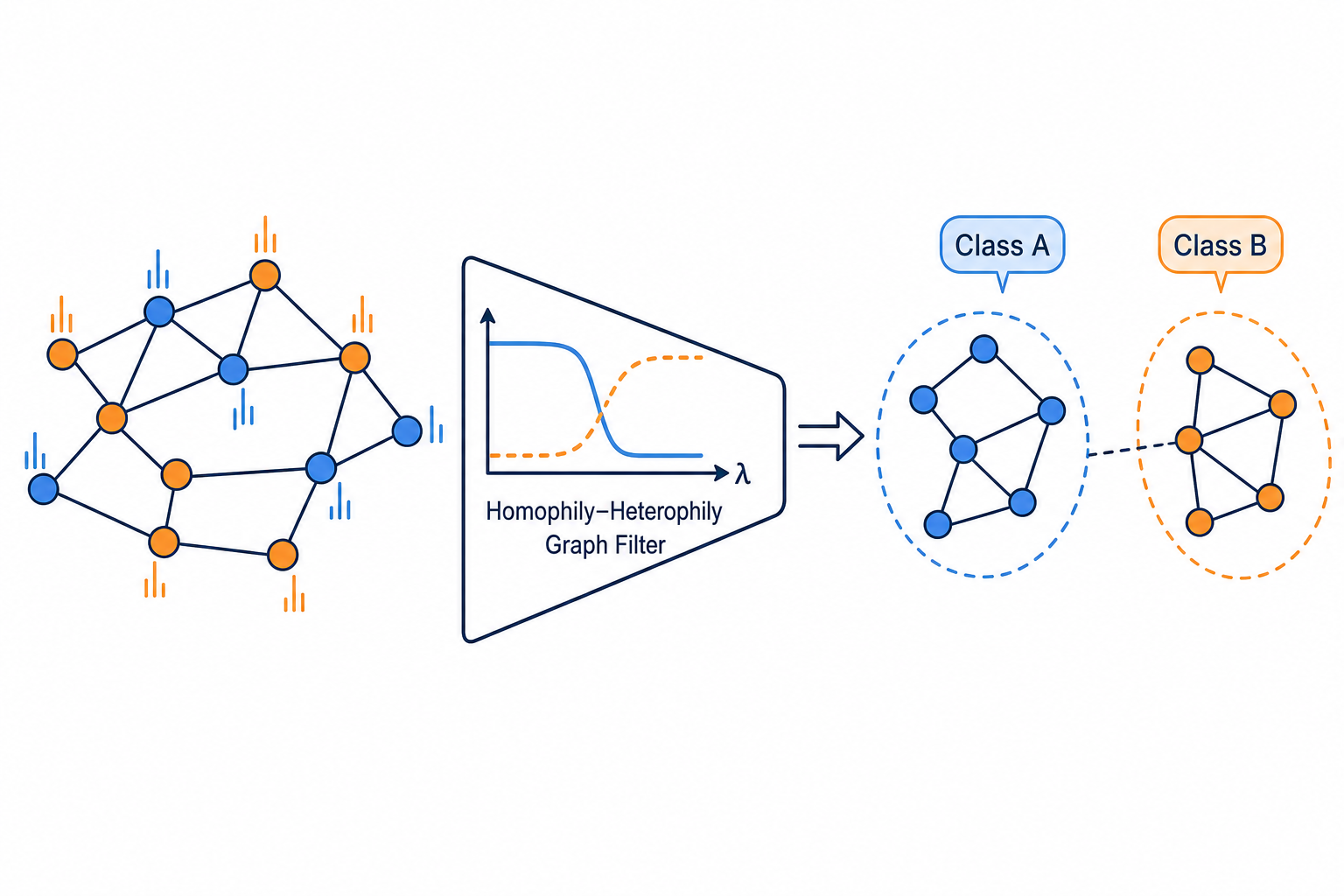
Homophily-Heterophily Graph Filter
The graph signal propagation filter is changed to improve node classification accuracy across homophilic and heterophilic graphs.
Description
Graph Signal Propagation: Spectral / Spatial Graph Filters
Research Question
Design a novel graph signal propagation filter for node feature aggregation in graph neural networks. The filter should effectively handle both homophilic graphs (where connected nodes share labels) and heterophilic graphs (where connected nodes often differ).
Background
GNNs propagate node features through graph structure using graph filters. The choice of filter is critical: simple low-pass filters such as GCN's first-order approximation work well on homophilic graphs but fail on heterophilic graphs, where useful information may live in higher-frequency components. Modern spectral methods learn polynomial filters in various bases:
- Monomial basis (GPRGNN):
h(A) = sum_k gamma_k A^k. Simple but can be numerically unstable. Chien, Peng, Li & Milenkovic, "Adaptive Universal Generalized PageRank Graph Neural Network," ICLR 2021 (arXiv:2006.07988). - Bernstein basis (BernNet): non-negative, excellent controllability, but
O(K^2)complexity. He, Wei, Huang & Xu, "BernNet: Learning Arbitrary Graph Spectral Filters via Bernstein Approximation," NeurIPS 2021 (arXiv:2106.10994). - Chebyshev interpolation (ChebNetII): avoids the Runge phenomenon,
O(K)complexity. He, Wei & Wen, "Convolutional Neural Networks on Graphs with Chebyshev Approximation, Revisited," NeurIPS 2022 (arXiv:2202.03580). - Jacobi polynomials (JacobiConv): orthogonal, fast convergence, generalizes Chebyshev / Legendre. Wang & Zhang, "How Powerful are Spectral Graph Neural Networks?", ICML 2022.
Key design axes include: polynomial basis choice, coefficient initialization and constraints, normalization (GCN vs Laplacian), and interaction with the MLP encoder.
Task
Modify the CustomProp (propagation layer) and CustomFilter (full model)
classes in custom_filter.py. The propagation layer defines how node features
are filtered across the graph; the model wraps it with an MLP encoder and
output head.
class CustomProp(MessagePassing):
    def __init__(self, K, alpha=0.1, **kwargs):
        # K: polynomial order, alpha: teleport probability
        ...
    def forward(self, x, edge_index, edge_weight=None):
        # x: [num_nodes, channels], edge_index: [2, num_edges]
        # returns filtered features [num_nodes, channels]
        ...


class CustomFilter(nn.Module):
    def __init__(self, num_features, num_classes, hidden=64, K=10,
                 alpha=0.1, dropout=0.5, dprate=0.5):
        ...
    def forward(self, data):
        # data: PyG Data object with data.x, data.edge_index
        # returns log_softmax predictions [num_nodes, num_classes]
        ...
Available utilities:
gcn_norm(edge_index)-- GCN normalizationD^{-1/2} A D^{-1/2}.get_laplacian(edge_index, normalization='sym')-- symmetric normalized LaplacianL = I - D^{-1/2} A D^{-1/2}.add_self_loops(edge_index, edge_weight, fill_value)-- add self loops.self.propagate(edge_index, x=x, norm=norm)-- single-step message passing.cheby(i, x)-- evaluate the Chebyshev polynomialT_i(x).comb(n, k)-- binomial coefficient (from scipy).- Constants:
K,ALPHA,HIDDEN,DROPOUT,DPRATE.
Evaluation
Datasets (a mix of homophilic and heterophilic graphs):
| Label | Nodes | Classes | Type | Source |
|---|---|---|---|---|
| cora | 2,708 | 7 | homophilic | citation network |
| citeseer | 3,327 | 6 | homophilic | citation network |
| texas | 183 | 5 | heterophilic | WebKB webpage network |
| cornell | 183 | 5 | heterophilic | WebKB webpage network |
Fixed pipeline: each dataset runs 10 random 60/20/20 train/val/test splits with early stopping.
Metric: mean test accuracy over the 10 runs, higher-is-better.
The contribution should remain a modular graph filter paired with the fixed classification pipeline, rather than changing the data split or evaluation target.
Code
1# Custom graph signal propagation filter for MLS-Bench2#3# EDITABLE section: CustomProp (propagation layer) + CustomFilter (full model).4# FIXED sections: everything else (config, data loading, training loop, evaluation).56import os7import math8import random9import time10from typing import Optional1112import numpy as np13import torch14import torch.nn as nn15import torch.nn.functional as F
Method Summary
Dual-Path Polynomial + Residual Gate
Two GPRGNN-style monomial filters (uniform-init + PPR-init) mixed by a learnable scalar, with a sigmoid residual gate to the unfiltered features.