3D Gaussian Splatting Densification Strategy Design

Objective

Design a densification strategy for 3D Gaussian Splatting (3DGS) that achieves the best novel view synthesis quality on real-world scenes.

Background

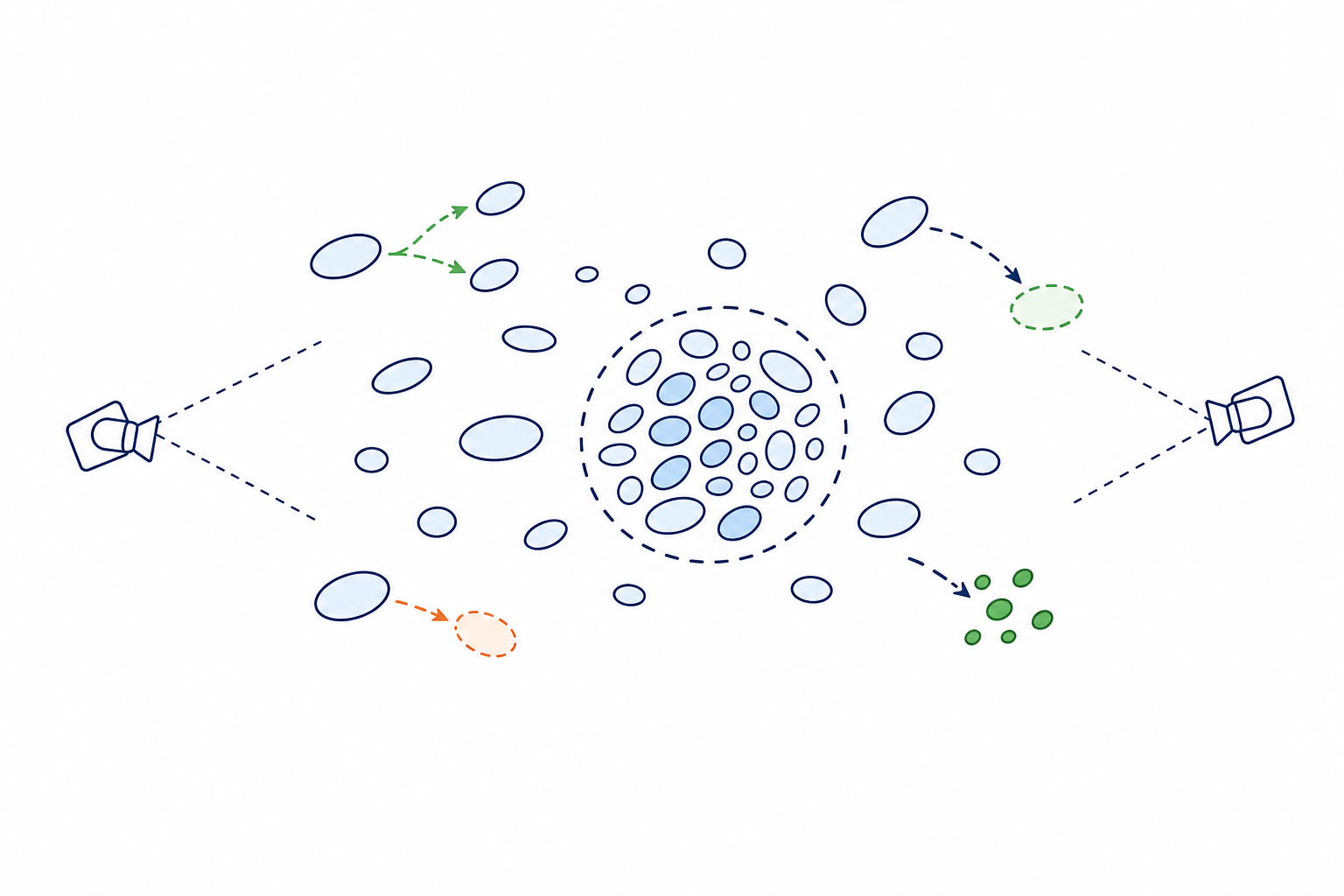
3D Gaussian Splatting represents scenes as collections of 3D Gaussians optimized via differentiable rendering. A critical component is the densification strategy, which controls how Gaussians are added, split, and pruned during optimization:

• Clone: Duplicate small Gaussians in under-reconstructed regions
• Split: Divide large Gaussians into smaller ones for finer detail
• Prune: Remove transparent or oversized Gaussians
• Reset: Periodically reset opacities to encourage pruning of unneeded Gaussians

Recent work has proposed various improvements:

• AbsGS: Uses absolute gradients instead of average for better detail recovery
• Mini-Splatting: Blur-aware forced splitting + importance-based pruning
• MCMC 3DGS: Treats densification as Markov Chain Monte Carlo sampling
• New Split (Cao et al.): Mathematically consistent Gaussian splitting

Task

Implement a CustomStrategy class in custom_strategy.py. Your strategy controls the full lifecycle of Gaussians during training via two hooks:

Editable Region

@dataclass
class CustomStrategy(Strategy):
    def initialize_state(self, scene_scale: float = 1.0) -> Dict[str, Any]:
        # Initialize running statistics for your strategy
        ...

    def step_pre_backward(self, params, optimizers, state, step, info):
        # Called BEFORE loss.backward(). Use to retain gradients.
        ...

    def step_post_backward(self, params, optimizers, state, step, info, packed=False):
        # Called AFTER loss.backward() and optimizer.step().
        # This is where you implement densification logic.
        ...

Available Operations (from gsplat.strategy.ops)

• duplicate(params, optimizers, state, mask) — Clone selected Gaussians
• split(params, optimizers, state, mask) — Split selected Gaussians (sample 2 new positions from covariance)
• remove(params, optimizers, state, mask) — Remove selected Gaussians
• reset_opa(params, optimizers, state, value) — Reset all opacities to a value
• relocate(params, optimizers, state, mask, binoms, min_opacity) — Teleport dead Gaussians to live ones
• sample_add(params, optimizers, state, n, binoms, min_opacity) — Add new Gaussians sampled from opacity distribution
• inject_noise_to_position(params, optimizers, state, scaler) — Perturb positions

Available Information

The info dict from rasterization contains:

• means2d: 2D projected means (with .grad after backward)
• width, height: Image dimensions
• n_cameras: Number of cameras in batch
• radii: Screen-space radii per Gaussian
• gaussian_ids: Which Gaussians are visible

The params dict contains Gaussian parameters:

• means: [N, 3] positions
• scales: [N, 3] log-scales
• quats: [N, 4] rotation quaternions
• opacities: [N] logit-opacities (use torch.sigmoid() for actual opacity)
• sh0, shN: Spherical harmonic coefficients for color

Architecture (Fixed)

• Renderer: gsplat CUDA rasterizer
• Optimizer: AdamW with per-parameter learning rates
• Loss: 0.8 × L1 + 0.2 × SSIM (fixed)
• Training: 30,000 steps per scene
• SH degree: 3 (increased gradually)

Evaluation

Novel view synthesis quality on held-out test views:

Evaluated on 4 Mip-NeRF 360 scenes (garden, bicycle, bonsai, stump) with every 8th image held out for testing.

Baselines

Reference Baseline PSNRs (MipNeRF360)

Your goal: beat the best baseline per-scene. taming leads on 3 of 4 scenes (garden / bicycle / bonsai); absgrad still leads stump by a narrow margin.