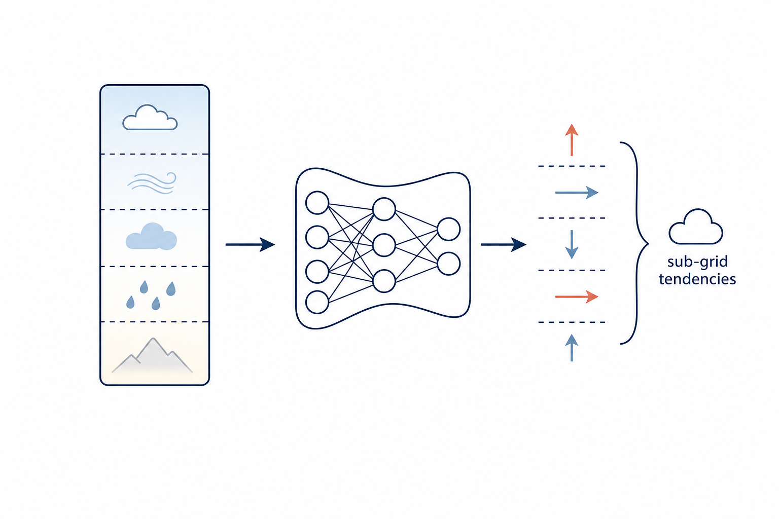
Atmospheric Column Emulator Architecture
Studies how neural emulator architecture maps vertical atmospheric states to sub-grid physics tendencies across training budgets.
Description
Climate Physics Emulation: Neural Network Architecture
Research Question
Design an improved neural network architecture for emulating sub-grid atmospheric physics processes in climate models. Your architecture should achieve lower Normalized MSE (NMSE) than the default MLP baseline on the ClimSim low-resolution dataset.
Background
Global climate models divide the atmosphere into grid cells, but many critical physical processes (radiation, convection, cloud formation) occur at scales smaller than these grid cells. Traditionally, these sub-grid processes are approximated by parameterization schemes — handcrafted physics-based approximations. Neural network emulators can learn these mappings from high-resolution simulation data, potentially improving both accuracy and computational efficiency.
ClimSim (Yu et al., "ClimSim: A large multi-scale dataset for hybrid physics-ML climate emulation", NeurIPS 2023 Datasets & Benchmarks; arXiv:2306.08754) provides data from the E3SM-MMF multi-scale climate model, where each sample maps an atmospheric column state to the corresponding sub-grid physics tendencies computed by the high-resolution physics module.
Task
Modify the Custom model class in custom_emulator.py to implement a better neural network architecture. The model must:
- Accept
input_dimandoutput_dimin__init__. - Implement
forward(x)wherexhas shape(batch_size, input_dim). - Return predictions of shape
(batch_size, output_dim).
Interface
Input structure (556-dim vector per atmospheric column):
- 9 multi-level variables × 60 vertical levels = 540 features:
temperature (
state_t), specific humidity (state_q0001), cloud ice (state_q0002), cloud liquid (state_q0003), zonal wind (state_u), meridional wind (state_v), ozone (pbuf_ozone), methane (pbuf_CH4), nitrous oxide (pbuf_N2O). - 16–17 single-level (surface/TOA) scalar variables: surface pressure, solar insolation, heat fluxes, wind stress, albedos, surface type fractions, snow depths.
Output structure (368-dim vector):
- 6 multi-level tendency variables × 60 levels = 360 features:
temperature tendency (
ptend_t), humidity tendencies (ptend_q0001–q0003), wind tendencies (ptend_u,ptend_v). - 8 single-level diagnostic outputs: net shortwave, longwave down, snow/rain precipitation, direct/diffuse solar.
Fixed Pipeline
Dataset loading, input/output normalization, train/val/test splits, optimizer choice and schedule, loss function, and the multi-budget evaluation harness are all fixed by the scaffold. Only the Custom architecture is editable.
Evaluation
- Primary metric: Normalized MSE (NMSE = MSE / Var(target), lower is better).
- Secondary metrics: R² (higher is better), RMSE, plus separate
ml_nmse(multi-level) andsl_nmse(single-level) breakdowns. - Training budgets: 30 epochs (short), 100 epochs (medium), 200 epochs (long).
- All three training budgets are run; improvements should be consistent across all three.
Reference Baselines
- cnn: 1D convolutional network with residual blocks operating on vertical atmospheric profiles. Multi-level variables are treated as spatial sequences over 60 vertical levels; single-level scalars are broadcast and concatenated. Inspired by the ClimSim CNN baseline (Yu et al., NeurIPS 2023 D&B).
- ed: Encoder-decoder (ClimSim ED baseline). Wide 6-layer fully-connected encoder compresses the 556-dim atmospheric state to a 5-node latent bottleneck, then a symmetric 6-layer decoder expands back to the 368-dim tendency output. Layer widths follow the published ClimSim Table A (768/512/384/256/128/64).
- unet: 1D U-Net with ResNet-style blocks over 60 vertical levels. Encoder-decoder with skip connections and self-attention at the bottleneck. Adapted from the ClimSim-style stable-ML-parameterization U-Net (arXiv:2407.00124).
- hsr: Heteroskedastic regression (ClimSim HSR baseline). Shared MLP backbone with two output heads predicting mean and log-variance per output dimension, trained with Gaussian NLL loss (Nix & Weigend 1994). Inference returns only the mean.
Code
1"""Custom Climate Physics Emulator2Trained on ClimSim low-resolution E3SM data to predict sub-grid physics tendencies.34Input: 556-dim atmospheric state vector (V2 variables)5Output: 368-dim sub-grid physics tendencies6"""78import math9import os10import time11from dataclasses import dataclass1213import numpy as np14import torch15import torch.nn as nn
1import xarray as xr2import numpy as np3import pandas as pd4import matplotlib.pyplot as plt5import pickle6import glob, os7import re8import tensorflow as tf9import netCDF410import copy11import string12import h5py13from tqdm import tqdm14from typing import Literal15
Method Summary
Gated multi-scale FiLM CNN
1D residual CNN over vertical levels with multi-scale gated convolutions, FiLM scalar conditioning, and SE channel attention.
1. split input into ml profile (9x60) and scalars s2. h ← Conv1d-stem(concat(ml, scalar->2x60 proj))3. for i = 1..8: if i ∈ FiLM points: h ← (1 + ) ⊙ h +4. h ← GatedResBlock with kernels {3, 5} and learned gate5. h ← h ⊙6. ml_out ← ML head; sl_out ← SL head + linear skip from s